Unit 1 Introduction to Diffusers
这个部分针对于如何使用 Diffusers 库来在数据上创建和训练自己的扩散模型。
1.1 怎么利用现有模型生成图片
利用 Hugging Face 的 diffusers 库,快速加载并部署一个特定微调模型(Stable Diffusion)的标准流程。其核心目的是构建一个文本生成图像的 Pipeline
首先从 diffusers 库中导入 StableDiffusionPipeline 类,这是运行扩散模型的标准接口。接着,通过指定 model_id,明确了要加载的模型来源。
注意一下这里的模型是针对这个动漫角色进行微调后的模型
from_pretrained 方法的调用,其中包含两个至关重要的参数。首先,torch_dtype=torch.float16 指定模型以半精度浮点数加载,这能显著降低显存占用并提升推理速度;其次,.to(device) 将模型直接部署到计算设备(如 GPU)上,确保图像生成过程的高效运算。
导入相应的模型之后,我们就可以通过给入相应的模型来生成相应的图片
这个模型是针对一个土豆动漫角色的一个微调,这时模型就知道 potato head 是什么东西了。这时给出这个 prompt,我们就可以得到我们相应的动漫角色了
from diffusers import StableDiffusionPipeline

# Check out https://huggingface.co/sd-dreambooth-library for loads of models from the community
model_id = "sd-dreambooth-library/mr-potato-head"

# Load the pipeline
pipe = StableDiffusionPipeline.from_pretrained(model_id, torch_dtype=torch.float16).to(
    device
)

prompt = "an abstract oil painting of sks mr potato head by picasso"
image = pipe(prompt, num_inference_steps=50, guidance_scale=7.5).images[0]
1.2 训练一个自己的 DDPMPipeline
接下来我们将深入探究这个扩散模型是怎么被训练出来的,这里我们要训练一个 DDPMPipeline,当然这个库中有现成的工具用于导入已训练好的模型,用于无条件图像生成,步骤与前面的 StableDiffusion 是类似的,只是我这里不需要输入 Prompt,因为这个生图过程是由噪声生成出来的。
from diffusers import DDPMPipeline

# Load the butterfly pipeline
butterfly_pipeline = DDPMPipeline.from_pretrained(
    "johnowhitaker/ddpm-butterflies-32px"
).to(device)

# Create 8 images
images = butterfly_pipeline(batch_size=8).images

# View the result
make_grid(images)
接下来我们将开始训练这样的一个模型。对于一个完整的扩散模型应用来说,有三个核心的组件
- Pipeline (流水线) 负责协调整个图像生成或训练的流程。目标是让用户能用最简单的代码完成复杂的任务。你只需要调用
pipe(),它内部就会自动执行文本编码、噪声生成、迭代去噪、图像解码等一系列繁琐的步骤。 - Model (模型) 负责进行具体的预测工作,例如预测图像中的噪声。
- Scheduler (调度器) 定义了去噪或加噪的具体规则和步骤。
散模型的训练流程主要包含以下几个循环步骤:
- 首先加载训练图像并添加不同程度的噪声
- 接着将这些带噪图像输入模型以评估其去噪能力
- 最后根据评估结果更新模型权重。
1.2.1 加载数据
首先我们需要加载训练数据
import torchvision
from datasets import load_dataset
from torchvision import transforms

dataset = load_dataset("huggan/smithsonian_butterflies_subset", split="train")

# 从本地的数据库中导入相应的数据
# dataset = load_dataset("imagefolder", data_dir="path/to/folder")

# 训练的图片变成为 32
image_size = 32
# batch_size 是一次训练要导入多少图片到 GPU 中进行一次训练
batch_size = 64

# Define data augmentations
# 定义数据增强的理财
preprocess = transforms.Compose(
    [
        transforms.Resize((image_size, image_size)),  # 将数据调整大小到 image_size
        transforms.RandomHorizontalFlip(),  # 以一定概率对图片进行左右翻转
        transforms.ToTensor(),  # 该函数将图片从 (H, W, C) 格式转换为 (C, H, W) 格式,将数据类型转为浮点型,并将像素值从 0-255 缩放到 0.0-1.0 范围。
        transforms.Normalize([0.5], [0.5]),  # 映射到 (-1, 1)
    ]
)

# examples 通常是一个包含原始数据的字典,比如 {"image": [...], "label": [...]}
def transform(examples):
    images = [preprocess(image.convert("RGB")) for image in examples["image"]]
    return {"images": images}

# set_transform 是 Dataset 对象的一个成员方法。
# 可以 “即时”地应用数据处理逻辑。也就是说,它不会修改硬盘上的原始数据,也不会立刻把所有数据都处理完存到内存里,而是当你通过索引(如 dataset[0])或 DataLoader 读取数据时,它才动态地调用你定义的函数进行处理。
dataset.set_transform(transform)

# Create a dataloader from the dataset to serve up the transformed images in batches
train_dataloader = torch.utils.data.DataLoader(
    dataset, batch_size=batch_size, shuffle=True
)
关于 Datasets 的用法
1.2.2 定义 Scheduler
接下来我们要定义 Scheduler,它负责在训练和推理的过程中,精确地控制 “什么时候加多少噪音”
- 训练阶段(Forward Process - 加噪):输入一张干净的图片,逐渐给它添加噪音,直到变成一张完全随机的噪点图。调度器决定在第 1 步、第 500 步、第 1000 步分别加多少噪音。
- 推理/生成阶段(Reverse Process - 去噪):从一张随机噪点图开始,模型一步步预测并移除噪音,最终还原出一张清晰的图片。调度器用于根据模型的预测,一步步指导图片如何“净化”。
DDPM
Denoising Diffusion Probabilistic Models(去噪扩散概率模型)这是扩散模型领域最经典的论文之一,奠定了现代扩散模型的基础算法。代码中使用的 DDPMScheduler 就是基于这篇论文实现的算法。
我们从 diffusers 库中导入 DDPM Scheduler 类,DDPMScheduler(num_train_timesteps=1000) 创建一个调度器的实例,其中整个加噪或去噪的过程被分成了 1000 个小步骤。步数越多,过程越细腻,但计算量也越大。
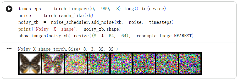
利用 noise_scheduler 完成对图片的加噪过程
1.2.3 定义模型
然后我们需要定义这个模型,也是整个部分的核心。大多数扩散模型使用的架构都是 U 型网络的某种变体,这也是我们这里要采用的架构。
首先通过绿色的下采样模块(Downsample)逐步压缩图像分辨率(从128x128逐级降至4x4),再经由橙色的中间模块(Middle block)处理后,通过粉色的上采样模块(Upsample)逐步还原分辨率至原始大小;
模型内部由多组ResNet层构成,每组下采样后图像尺寸减半,随后通过相同数量的上采样模块恢复尺寸,并利用跳跃连接(skip connections)将下采样路径的特征传递至上采样路径以保留细节;
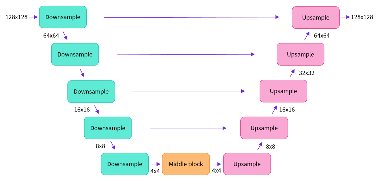
Diffusers库提供了UNet2DModel类,可直接在PyTorch中构建这一结构,其中down_block_types和up_block_types参数分别对应图中绿色和粉色的模块类型
from diffusers import UNet2DModel

xb = next(iter(train_dataloader))["images"].to(device)[:8]
timesteps = torch.linspace(0, 999, 8).long().to(device)
noise = torch.randn_like(xb)

noisy_xb = noise_scheduler.add_noise(xb, noise, timesteps)

# Create a model
model = UNet2DModel(
    sample_size=image_size,  # the target image resolution
    in_channels=3,  # the number of input channels, 3 for RGB images
    out_channels=3,  # the number of output channels
    layers_per_block=2,  # how many ResNet layers to use per UNet block
    block_out_channels=(64, 128, 128, 256),  # More channels -> more parameters
    down_block_types=(
        "DownBlock2D",  # a regular ResNet downsampling block
        "DownBlock2D",
        "AttnDownBlock2D",  # a ResNet downsampling block with spatial self-attention
        "AttnDownBlock2D",
    ),
    up_block_types=(
        "AttnUpBlock2D",
        "AttnUpBlock2D",  # a ResNet upsampling block with spatial self-attention
        "UpBlock2D",
        "UpBlock2D",  # a regular ResNet upsampling block
    ),
)
model.to(device);
然后如何让模型输出预测添加的噪声长什么样子,给入加噪后的图片以及加噪的步数
.sample属性:diffusers库中的模型通常遵循统一的 API 设计,将预测结果封装在一个包含.sample属性的对象中返回。因此,你需要通过.sample来提取出这个预测的张量。
1.2.4 训练模型
那么模型定义好之后,我们就要开始训练这个模型了,一共训练 30 轮
# Set the noise scheduler
noise_scheduler = DDPMScheduler(
    num_train_timesteps=1000, beta_schedule="squaredcos_cap_v2"
)

# Training loop 定义优化器,输入的参数是要调整的参数以及学习率
optimizer = torch.optim.AdamW(model.parameters(), lr=4e-4)

# 用于记录每个 epoch 后 loss 的变化
losses = []

for epoch in range(30):
    for step, batch in enumerate(train_dataloader):
        clean_images = batch["images"].to(device)

        # 构建噪声
        noise = torch.randn(clean_images.shape).to(clean_images.device)
        # batch 大小
        bs = clean_images.shape[0]

        # 为 batch 中的每一个图都生成一个 timestep
        timesteps = torch.randint(
            0, noise_scheduler.num_train_timesteps, (bs,), device=clean_images.device
        ).long()

        # 给这个 batch 中的每个图片加上噪声
        noisy_images = noise_scheduler.add_noise(clean_images, noise, timesteps)

        # 得到预测的噪声
        noise_pred = model(noisy_images, timesteps, return_dict=False)[0]

        # 与原先的噪声做比较,计算 loss
        loss = F.mse_loss(noise_pred, noise)
        # 回传梯度
        loss.backward(loss)
        # 记录这轮训练之后 loss 的大小
        losses.append(loss.item())

        # 根据 Optimizer 对参数进行更新
        optimizer.step()
        optimizer.zero_grad()

    if (epoch + 1) % 5 == 0:
        loss_last_epoch = sum(losses[-len(train_dataloader) :]) / len(train_dataloader)
        print(f"Epoch:{epoch+1}, loss: {loss_last_epoch}")
复习一下这里 python 的语法
enumerate(...)返回的是一个元组 (index, element),其中index是当前是第几个元素(从0开始)以及 element是当前元素本身。
torch.randint 用于生成随机整数的函数。
-
范围参数:0, noise_scheduler.num_train_timesteps,左闭右开
-
形状参数:(bs,) 含义:定义输出张量的尺寸(Shape)。
-
设备参数:device=clean_images.device
1.2.5 使用模型产生图片
这样经过 30 轮的训练之后,我们就得到了训练好的 model 和 noise_scheduler。然后我们就可以将其作为参数添加到 DDPMPipeline 中去了,这样就得到了一个无条件图像生成器了
from diffusers import DDPMPipeline

image_pipe = DDPMPipeline(unet=model, scheduler=noise_scheduler)

pipeline_output = image_pipe()
pipeline_output.images[0]
我们也可以将这个 Pipeline 保存到本地,其中包含了 model_index.json scheduler unet 三个内容,unet 中保存了和模型相关的信息,有 config.json diffusion_pytorch_model.safetensors
image_pipe.save_pretrained("my_pipeline")

!ls my_pipeline/
-> model_index.json  scheduler  unet

!ls my_pipeline/unet/
-> config.json  diffusion_pytorch_model.safetensors
深入到这个 Pipeline 中的具体细节,实际上就是完成一个去噪的过程
# 从8张噪声图开始去噪
sample = torch.randn(8, 3, 32, 32).to(device)

for i, t in enumerate(noise_scheduler.timesteps):

    # Get model pred
    # 给模型当前的噪声,以及现在的时间步,预测噪声
    # 其中 noise_scheduler.timesteps 给的时间步是倒序的
    with torch.no_grad():
        residual = model(sample, t).sample

    # Update sample with step
    # 进行一步去噪,输入的参数是当前预测的操作,时间步,当前带噪图像,返回值在 prev_sample 上
    sample = noise_scheduler.step(residual, t, sample).prev_sample

show_images(sample)
如何将自己训练的 model 上传到 hugging face
from huggingface_hub import get_full_repo_name

model_name = "sd-class-butterflies-32"
hub_model_id = get_full_repo_name(model_name)
在 Hugging face 上创建一个 reposity ,并 push 上自己的 model
from huggingface_hub import HfApi, create_repo

create_repo(hub_model_id)
api = HfApi()
api.upload_folder(
    folder_path="my_pipeline/scheduler", path_in_repo="", repo_id=hub_model_id
)
api.upload_folder(folder_path="my_pipeline/unet", path_in_repo="", repo_id=hub_model_id)
api.upload_file(
    path_or_fileobj="my_pipeline/model_index.json",
    path_in_repo="model_index.json",
    repo_id=hub_model_id,
)
这样我们就可以让别人使用我们训练好的模型了
之前的代码是简化后的结果,省略了很多的工程细节(当然思想是一致的),为了让你能处理更大的模型和更多数据,脚本补充了以下关键功能:
- 多 GPU 支持:利用多块显卡加速训练。
- 日志记录:记录训练进度和生成的示例图片。
- 梯度检查点:节省显存,从而支持更大的批次大小。
- 自动上传模型:将训练好的模型自动推送到 Hugging Face Hub。
下载 训练代码 我们可以完成更大模型的训练
执行脚本
accelerate launch train_unconditional.py \
  --dataset_name="huggan/smithsonian_butterflies_subset" \
  --resolution=64 \
  --output_dir={model_name} \
  --train_batch_size=32 \
  --num_epochs=50 \
  --gradient_accumulation_steps=1 \
  --learning_rate=1e-4 \
  --lr_warmup_steps=500 \
  --mixed_precision="no"
accelerate launch:这是 Hugging Face 提供的一个神奇命令。它会自动检测你的硬件环境(比如有几块 GPU),并自动配置分布式训练、混合精度(FP16/FP32)等复杂设置,而你不需要修改代码。
然后和之前一样将训练好的模型上传到 Hugging face 仓库中即可
1.3 DDPM 论文阅读
评论区
对你有帮助的话请给我个赞和 star => 欢迎跟我探讨!!!