Unit 2 Fine-Tuning, Guidance and Conditioning

Fine-Tuning

微调的含义就是对已有的模型进行在新的数据上进行重新训练从而改变模型的输出。微调的过程和 Unit 1 中训练的过程是类似的，只是这里我们是从一个已经训练好的模型开始的。

首先导入要训练的数据

dataset_name = "huggan/anime-faces"  # @param
dataset = load_dataset(dataset_name, split="train")
image_size = 256  # @param
batch_size = 4  # @param
preprocess = transforms.Compose(
    [
        transforms.Resize((image_size, image_size)),
        transforms.RandomHorizontalFlip(),
        transforms.ToTensor(),
        transforms.Normalize([0.5], [0.5]),
    ]
)


def transform(examples):
    images = [preprocess(image.convert("RGB")) for image in examples["image"]]
    return {"images": images}


dataset.set_transform(transform)

train_dataloader = torch.utils.data.DataLoader(
    dataset, batch_size=batch_size, shuffle=True
)

由于我们这里每张图片的大小比较大，所以如果 batch 比较大的话就会导致显卡内存爆炸。但是每次四张照片计算的梯度误差太大，这里就有一个优化的技术，即 gradient accumulation。

在调用 optimizer.step() 更新参数和 optimizer.zero_grad() 清空梯度之前，连续多次执行 loss.backward()。PyTorch 会自动将这些梯度累加求和，从而将多个小批次的数据合并成一个“虚拟的大批次”来更新模型。这种做法不仅模拟了大 Batch Size 的训练效果，提供了更稳定的梯度估计

num_epochs = 2  # @param
lr = 1e-5  # @param
grad_accumulation_steps = 2  # @param

optimizer = torch.optim.AdamW(image_pipe.unet.parameters(), lr=lr)

losses = []

for epoch in range(num_epochs):
    for step, batch in tqdm(enumerate(train_dataloader), total=len(train_dataloader)):
        clean_images = batch["images"].to(device)
        # Sample noise to add to the images
        noise = torch.randn(clean_images.shape).to(clean_images.device)
        bs = clean_images.shape[0]

        # Sample a random timestep for each image
        timesteps = torch.randint(
            0,
            image_pipe.scheduler.num_train_timesteps,
            (bs,),
            device=clean_images.device,
        ).long()

        # Add noise to the clean images according to the noise magnitude at each timestep
        # (this is the forward diffusion process)
        noisy_images = image_pipe.scheduler.add_noise(clean_images, noise, timesteps)

        # Get the model prediction for the noise
        noise_pred = image_pipe.unet(noisy_images, timesteps, return_dict=False)[0]

        # Compare the prediction with the actual noise:
        loss = F.mse_loss(
            noise_pred, noise
        )  # NB - trying to predict noise (eps) not (noisy_ims-clean_ims) or just (clean_ims)

        # Store for later plotting
        losses.append(loss.item())

        # Update the model parameters with the optimizer based on this loss
        loss.backward(loss)

        # Gradient accumulation:
        if (step + 1) % grad_accumulation_steps == 0:
            optimizer.step()
            optimizer.zero_grad()

    print(
        f"Epoch {epoch} average loss:{sum(losses[len(train_dataloader):])/len(train_dataloader)}"
    )

# Plot the loss curve:
plt.plot(losses)

当然 Hugging face 也有相应的继承库 Accelerate 集成了这些功能可以直接调用。

对于聚焦于图像生成任务（如扩散模型）的微调（fine-tuning）实践。我们需要在模型训练的过程中进行监控和改进，需要吩咐的反馈机制来定性 + 定量地评估训练进展。

• 可以每隔若干 epoch，让模型生成一些图像样本，人工观察这些样本的变化趋势，从而直观判断模型是否在学习新数据分布；

• 记录关键训练日志（logging）记录 loss、生成样本、模型参数（如 weights & biases）、梯度等，可以使用工具 Weights & Biases（W&B）或 TensorBoard

微调效果的好坏高度依赖具体任务目标，因此“良好性能”的标准并不统一。

若在小规模数据集上微调一个文本条件生成模型（如 Stable Diffusion），通常希望模型保留对原始提示词的理解能力，此时应采用较低学习率并配合正则化手段（如指数移动平均）；

而如果目标是让模型彻底适应新数据分布（如从卧室图像转向 wikiart 艺术风格），则更适合使用较大学习率和更长训练时间，近乎重新训练。值得注意的是，即使 loss 曲线未明显下降，生成样本仍可能显示出模型正从原始域向新域迁移——图像逐渐呈现艺术风格但整体仍失真、不连贯。这一现象也引出了下一阶段的关键问题：如何通过额外的引导机制，实现对生成结果更精细的控制。

Guidance

为实现对生成样本的可控性，比如说指定输出图像颜色，可引入引导（guidance）技术

那么首先我们需要重新定义一个条件损失函数 color_loss，用于衡量生成图像像素与目标颜色（默认浅青色）之间的平均绝对误差；

def color_loss(images, target_color=(0.1, 0.9, 0.5)):
    """Given a target color (R, G, B) return a loss for how far away on average
    the images' pixels are from that color. Defaults to a light teal: (0.1, 0.9, 0.5)"""
    target = (
        torch.tensor(target_color).to(images.device) * 2 - 1
    )  # Map target color to (-1, 1)
    target = target[
        None, :, None, None
    ]  # Get shape right to work with the images (b, c, h, w)
    error = torch.abs(
        images - target
    ).mean()  # Mean absolute difference between the image pixels and the target color
    return error

接着在采样过程中修改迭代步骤——创建一个需计算梯度的噪声变量 x，先用 U-Net 预测去噪结果 x₀，再将其输入该损失函数，反向传播得到梯度，并用此梯度在 scheduler 更新前对 x 进行修正，从而“引导”生成方向朝向目标属性。

就是每次去噪前按照我设定的 gudiance 修正一下

这里有两种可选的实现方式：

• 第一种是在从 U-Net 获得噪声预测后再对变量 x 启用梯度（requires_grad=True），这种方式内存更高效（因为无需追踪扩散模型内部的梯度），但得到的梯度精度较低；

# Variant 1: shortcut method

# The guidance scale determines the strength of the effect
guidance_loss_scale = 40  # Explore changing this to 5, or 100

x = torch.randn(8, 3, 256, 256).to(device)

for i, t in tqdm(enumerate(scheduler.timesteps)):

    # Prepare the model input
    model_input = scheduler.scale_model_input(x, t)

    # predict the noise residual
    with torch.no_grad():
        noise_pred = image_pipe.unet(model_input, t)["sample"]

    # Set x.requires_grad to True
    x = x.detach().requires_grad_()

    # Get the predicted x0
    x0 = scheduler.step(noise_pred, t, x).pred_original_sample

    # Calculate loss
    loss = color_loss(x0) * guidance_loss_scale
    if i % 10 == 0:
        print(i, "loss:", loss.item())

    # Get gradient
    cond_grad = -torch.autograd.grad(loss, x)[0]

    # Modify x based on this gradient
    x = x.detach() + cond_grad

    # Now step with scheduler
    x = scheduler.step(noise_pred, t, x).prev_sample

• 第二种是先对 x 启用梯度，再将其输入 U-Net 并计算预测的 x₀，这样能获得更准确的梯度，但内存开销更大。

# Variant 2: setting x.requires_grad before calculating the model predictions

guidance_loss_scale = 40
x = torch.randn(4, 3, 256, 256).to(device)

for i, t in tqdm(enumerate(scheduler.timesteps)):

    # Set requires_grad before the model forward pass
    x = x.detach().requires_grad_()
    model_input = scheduler.scale_model_input(x, t)

    # predict (with grad this time)
    noise_pred = image_pipe.unet(model_input, t)["sample"]

    # Get the predicted x0:
    x0 = scheduler.step(noise_pred, t, x).pred_original_sample

    # Calculate loss
    loss = color_loss(x0) * guidance_loss_scale
    if i % 10 == 0:
        print(i, "loss:", loss.item())

    # Get gradient
    cond_grad = -torch.autograd.grad(loss, x)[0]

    # Modify x based on this gradient
    x = x.detach() + cond_grad

    # Now step with scheduler
    x = scheduler.step(noise_pred, t, x).prev_sample

CLIP Gudiance

CLIP Guidance 是一种利用 CLIP 模型实现文本引导图像生成的技术：

• 首先将文本提示编码为 512 维嵌入向量；
• 在扩散模型每一步采样中，对预测的去噪图像生成多个变体（增强多样性），分别用 CLIP 编码为图像嵌入，并与文本嵌入计算“大圆距离平方”（Great Circle Distance Squared）作为损失；
• 再反向传播该损失，得到对当前噪声状态 \(x\) 的梯度，用于在 scheduler 更新前修正 \(x\) ，从而引导生成结果更贴合文本描述。

# @markdown load a CLIP model and define the loss function
import open_clip

clip_model, _, preprocess = open_clip.create_model_and_transforms(
    "ViT-B-32", pretrained="openai"
)
clip_model.to(device)

# Transforms to resize and augment an image + normalize to match CLIP's training data
tfms = torchvision.transforms.Compose(
    [
        torchvision.transforms.RandomResizedCrop(224),  # Random CROP each time
        torchvision.transforms.RandomAffine(
            5
        ),  # One possible random augmentation: skews the image
        torchvision.transforms.RandomHorizontalFlip(),  # You can add additional augmentations if you like
        torchvision.transforms.Normalize(
            mean=(0.48145466, 0.4578275, 0.40821073),
            std=(0.26862954, 0.26130258, 0.27577711),
        ),
    ]
)

# And define a loss function that takes an image, embeds it and compares with
# the text features of the prompt
def clip_loss(image, text_features):
    image_features = clip_model.encode_image(
        tfms(image)
    )  # Note: applies the above transforms
    input_normed = torch.nn.functional.normalize(image_features.unsqueeze(1), dim=2)
    embed_normed = torch.nn.functional.normalize(text_features.unsqueeze(0), dim=2)
    dists = (
        input_normed.sub(embed_normed).norm(dim=2).div(2).arcsin().pow(2).mul(2)
    )  # Squared Great Circle Distance
    return dists.mean()

定义好指导的损失函数之后，之后的步骤和之前基本类似

# @markdown applying guidance using CLIP

prompt = "Red Rose (still life), red flower painting"  # @param

# Explore changing this
guidance_scale = 8  # @param
n_cuts = 4  # @param

# More steps -> more time for the guidance to have an effect
scheduler.set_timesteps(50)

# We embed a prompt with CLIP as our target
text = open_clip.tokenize([prompt]).to(device)
with torch.no_grad(), torch.cuda.amp.autocast():
    text_features = clip_model.encode_text(text)


x = torch.randn(4, 3, 256, 256).to(
    device
)  # RAM usage is high, you may want only 1 image at a time

for i, t in tqdm(enumerate(scheduler.timesteps)):

    model_input = scheduler.scale_model_input(x, t)

    # predict the noise residual
    with torch.no_grad():
        noise_pred = image_pipe.unet(model_input, t)["sample"]

    cond_grad = 0

    # 下面这一步就是在生成变体取平均，clip_loss 生成了图像变体，比如说裁剪、缩放、颜色抖动等，起到多视角评估的作用
    for cut in range(n_cuts):

        # Set requires grad on x
        x = x.detach().requires_grad_()

        # Get the predicted x0:
        x0 = scheduler.step(noise_pred, t, x).pred_original_sample

        # Calculate loss
        loss = clip_loss(x0, text_features) * guidance_scale

        # Get gradient (scale by n_cuts since we want the average)
        cond_grad -= torch.autograd.grad(loss, x)[0] / n_cuts

    if i % 25 == 0:
        print("Step:", i, ", Guidance loss:", loss.item())

    # Modify x based on this gradient
    alpha_bar = scheduler.alphas_cumprod[i]
    x = (
        x.detach() + cond_grad * (1-alpha_bar).sqrt()
    )  # Note the additional scaling factor here!

    # Now step with scheduler
    x = scheduler.step(noise_pred, t, x).prev_sample

在扩散模型的引导生成过程中，对条件梯度（conditioning gradient）施加一个时间相关的缩放因子（如代码中的 (1 - alpha_bar).sqrt()）是一种关键技巧。

alpha_bar 是累积方差项，随去噪步数增加而减小，因此该因子使得早期步骤的引导强度较弱，后期逐步增强。虽然存在理论分析建议“最优”缩放方式，但实践中这一调度策略高度依赖任务目标：例如，若引导目标是整体语义（如物体类别），可能希望早期强引导以确立结构；而若关注局部纹理或风格细节，则更适合后期介入，避免过早约束破坏全局布局。

因此，开发者常通过实验调整梯度缩放的时间调度（schedule），以平衡生成质量与条件对齐效果。

---

实际应用中的 CLIP 引导扩散（CLIP-guided diffusion）远比简易示例复杂：成熟的实现通常包含专门的随机裁剪（random cutouts）模块，从生成图像中采样多个不同尺度和位置的局部视图，并结合多种针对 CLIP 特性的损失函数优化技巧（如归一化、温度缩放、多层特征融合等），以显著提升文本-图像对齐效果。

在文生图扩散模型（如 DALL·E 2、Stable Diffusion）出现之前，CLIP 引导扩散曾是最强大的文本到图像生成方法。尽管当前这个“玩具版”实现较为简略、性能有限，但它清晰地体现了核心思想：借助梯度引导机制和 CLIP 强大的跨模态语义对齐能力，我们可以在一个原本无条件的扩散模型上，动态注入文本控制信号，从而实现高质量的文本引导图像生成。

Conditioning

在 Unit 1 中我们训练出了一个能输出手写字的扩散模型，但是输出的图片我们并不知道它会是哪个数字，那么我们能否给他加上限制 (Class-Conditioned)，让它根据我们生成我们想要的手写数字呢？

首先加载训练数据

# Load the dataset
dataset = torchvision.datasets.MNIST(root="mnist/", train=True, download=True, transform=torchvision.transforms.ToTensor())

# Feed it into a dataloader (batch size 8 here just for demo)
train_dataloader = DataLoader(dataset, batch_size=8, shuffle=True)

然后我们希望把每张图片和相应的数字都输入到模型中

首先通过embedding 层将类别标签映射为一个可学习的向量，然后将该向量重塑并扩展为与输入图像相同的空间尺寸，最后将其作为额外的通道与原始图像在通道维度上拼接，形成包含类别信息的输入张量，再送入 U-Net 进行预测。

其中嵌入向量的维度（class_emb_size）是可调的超参数，也可尝试使用独热编码等替代方案。

class ClassConditionedUnet(nn.Module):
  def __init__(self, num_classes=10, class_emb_size=4):
    super().__init__()

    # The embedding layer will map the class label to a vector of size class_emb_size
    self.class_emb = nn.Embedding(num_classes, class_emb_size)

    # Self.model is an unconditional UNet with extra input channels to accept the conditioning information (the class embedding)
    self.model = UNet2DModel(
        sample_size=28,           # the target image resolution
        in_channels=1 + class_emb_size, # Additional input channels for class cond.
        out_channels=1,           # the number of output channels
        layers_per_block=2,       # how many ResNet layers to use per UNet block
        block_out_channels=(32, 64, 64), # 指的是每一层的通道数
        down_block_types=(
            "DownBlock2D",        # a regular ResNet downsampling block
            "AttnDownBlock2D",    # a ResNet downsampling block with spatial self-attention
            "AttnDownBlock2D",
        ),
        up_block_types=(
            "AttnUpBlock2D",
            "AttnUpBlock2D",      # a ResNet upsampling block with spatial self-attention
            "UpBlock2D",          # a regular ResNet upsampling block
          ),
    )

  # Our forward method now takes the class labels as an additional argument
  def forward(self, x, t, class_labels):
    # Shape of x:
    bs, ch, w, h = x.shape

    # class conditioning in right shape to add as additional input channels
    class_cond = self.class_emb(class_labels) # Map to embedding dimension
    class_cond = class_cond.view(bs, class_cond.shape[1], 1, 1).expand(bs, class_cond.shape[1], w, h)
    # x is shape (bs, 1, 28, 28) and class_cond is now (bs, 4, 28, 28)

    # Net input is now x and class cond concatenated together along dimension 1
    net_input = torch.cat((x, class_cond), 1) # (bs, 5, 28, 28)

    # Feed this to the UNet alongside the timestep and return the prediction
    return self.model(net_input, t).sample # (bs, 1, 28, 28)

其实就是把 label 的信息增加到图片的通道上了，然后接着完成训练的过程。

# Create a scheduler
noise_scheduler = DDPMScheduler(num_train_timesteps=1000, beta_schedule='squaredcos_cap_v2')

#@markdown Training loop (10 Epochs):

# Redefining the dataloader to set the batch size higher than the demo of 8
train_dataloader = DataLoader(dataset, batch_size=128, shuffle=True)

# How many runs through the data should we do?
n_epochs = 10

# Our network
net = ClassConditionedUnet().to(device)

# Our loss function
loss_fn = nn.MSELoss()

# The optimizer
opt = torch.optim.Adam(net.parameters(), lr=1e-3)

# Keeping a record of the losses for later viewing
losses = []

# The training loop
for epoch in range(n_epochs):
    for x, y in tqdm(train_dataloader):

        # Get some data and prepare the corrupted version
        x = x.to(device) * 2 - 1 # Data on the GPU (mapped to (-1, 1))
        y = y.to(device)
        noise = torch.randn_like(x)
        timesteps = torch.randint(0, 999, (x.shape[0],)).long().to(device)
        noisy_x = noise_scheduler.add_noise(x, noise, timesteps)

        # Get the model prediction
        # 输入的时候加入 labels 的信息
        pred = net(noisy_x, timesteps, y) # Note that we pass in the labels y

        # Calculate the loss
        loss = loss_fn(pred, noise) # How close is the output to the noise

        # Backprop and update the params:
        opt.zero_grad()
        loss.backward()
        opt.step()

        # Store the loss for later
        losses.append(loss.item())

    # Print out the average of the last 100 loss values to get an idea of progress:
    avg_loss = sum(losses[-100:])/100
    print(f'Finished epoch {epoch}. Average of the last 100 loss values: {avg_loss:05f}')

# View the loss curve
plt.plot(losses)

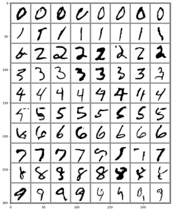
训练完成之后，我们就可以指定要生成的手写数字了

#@markdown Sampling some different digits:

# Prepare random x to start from, plus some desired labels y
x = torch.randn(80, 1, 28, 28).to(device)
y = torch.tensor([[i]*8 for i in range(10)]).flatten().to(device)

# Sampling loop
for i, t in tqdm(enumerate(noise_scheduler.timesteps)):

    # Get model pred
    with torch.no_grad():
        residual = net(x, t, y)  # Again, note that we pass in our labels y

    # Update sample with step
    x = noise_scheduler.step(residual, t, x).prev_sample

# Show the results
fig, ax = plt.subplots(1, 1, figsize=(12, 12))
ax.imshow(torchvision.utils.make_grid(x.detach().cpu().clip(-1, 1), nrow=8)[0], cmap='Greys')

评论区

对你有帮助的话请给我个赞和 star =>
欢迎跟我探讨！！！